This page was generated from docs/Examples/4d. other_isobar.ipynb. Interactive online version: .

Python Notebook Download

4d. Calculate isobars and isopleths

This allows you to calculate H2O-CO2 isobars and isopleths for a given melt composition and temperature.

Python set-up

You need to install VolFe once on your machine, if you haven’t yet. Then we need to import a few Python packages (including VolFe).

# Install VolFe on your machine. Don't remove the # from this line!
# pip install VolFe # Remove the first # in this line if you have not installed VolFe on your machine before.

# import python packages
import pandas as pd
import matplotlib.pyplot as plt
import VolFe as vf

Check version

vf.__version__

'1.0.2'

Define inputs

The melt composition and temperature can be given in a dataframe, or read from a csv file.

In this example it is read from a dataframe,which is from Brounce et al. (2014) with the updated Fe3+/FeT from Cottrell et al. (2021).

Note the volatile content of the melt is not used in this calculation.

# Define the melt composition, fO2 estimate, and T as a dictionary.
my_analysis = {'Sample':'Sari15-04-33',
           'T_C': 1200., # Temperature in 'C
           'SiO2': 47.89, # wt%
           'TiO2': 0.75, # wt%
           'Al2O3': 16.74, # wt%
           'FeOT': 9.43, # wt%
           'MnO': 0.18, # wt%
           'MgO': 5.92, # wt%
           'CaO': 11.58, # wt%
           'Na2O': 2.14, # wt%
           'K2O': 0.63, # wt%
           'P2O5': 0.17, # wt%
           'Fe3FeT': 0.177}

# Turn the dictionary into a pandas dataframe, setting the index to 0.
my_analysis = pd.DataFrame(my_analysis, index=[0])

We’ll mostly use the default options…

# print default options in VolFe
print(vf.default_models)

                            option
type
COH_species     yes_H2_CO_CH4_melt
H2S_m                         True
species X                       Ar
Hspeciation                   none
fO2                       Kress91A
...                            ...
error                          0.1
print status                 False
output csv                    True
setup                        False
high precision               False

[78 rows x 1 columns]

… but the ‘COH_species’ must be set to ‘H2O-CO2 only’ because the isobars and isopleths are calculated assuming the only melt and vapor species are H2O and CO2O.

# change just the "COH_species" option to "H2O-CO2 only"
my_models = [['COH_species','H2O-CO2 only']]

# turn "my_models" to dataframe with correct column headers and indexes
my_models = vf.make_df_and_add_model_defaults(my_models)

Run calculations

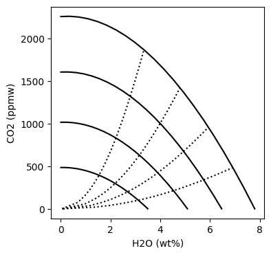
The isobar calculation is run as below. The initial and final pressure, as well as the pressure step, can be specified.

# calculate isobars starting at 1000 bars, ending at 4000 bars at 1000 bar intervals
isobars = vf.calc_isobar(my_analysis,models=my_models,initial_P=1000.,final_P=4000.,step_P=1000.)

The isopleth calculation is run as below. The highest pressure, as well as the step-size for the H2O mole fraction in the vapor, can be specified.

# calculate isopleths up to 4000 bar, at XH2O = 0.20 stepsizes
isopleths = vf.calc_isopleth(my_analysis,models=my_models,final_P=4000.,step_XH2O=0.10)

Plotting

And we can plot them

fig, (ax1) = plt.subplots(1, 1, figsize=(4,4))

# Plotting results
for P in [1000,2000,3000,4000]:
    df = isobars[isobars["P_bar"]==P]
    ax1.plot(df['H2O_wtpc'], df['CO2_ppm'], '-k')
for XH2O in [0.2,0.4,0.6,0.8]:
    df = isopleths[isopleths["XH2O"]==XH2O]
    if XH2O == 0.6:
        df = isopleths[isopleths["XH2O"]<0.7]
        df = df[df["XH2O"]>0.5]
    ax1.plot(df['H2O_wtpc'], df['CO2_ppm'], ':k')

ax1.set_ylabel('CO2 (ppmw)')
ax1.set_xlabel('H2O (wt%)')

Text(0.5, 0, 'H2O (wt%)')