This page was generated from
docs/Examples/1c. pvsat user_opt.ipynb.
Interactive online version:
![]() .
.
1c. Calculate Pvsat for analyses in a csv file using user specified options
What if I don’t want to use the default options…
Python set-up
You need to install VolFe once on your machine, if you haven’t yet. Then we need to import a few Python packages (including VolFe).
[1]:
# Install VolFe on your machine. Don't remove the # from this line!
# pip install VolFe # Remove the first # in this line if you have not installed VolFe on your machine before.

# import python packages
import pandas as pd
import matplotlib.pyplot as plt
import VolFe as vf
Define the inputs
In that case, we create a dataframe telling VolFe what to use instead. There are lots of options that can be changed, which can be viewed below or in the API reference section on the ReadTheDocs.
[2]:
help(vf.make_df_and_add_model_defaults)
Help on function make_df_and_add_model_defaults in module VolFe.model_dependent_variables:

make_df_and_add_model_defaults(models)
    Converts user-provided model configurations (e.g. ['carbon dioxide','MORB_Dixon95'],['hydrogen sulfide','basaltic andesite']
    into a structured pandas DataFrame, combined with default options for anything not specified


    Parameters
    ----------
    models : list of [str, str]
        A list of lists, where each inner list contains two elements: the model type (str)
        and the user-specified option (str) for that model type.

    Returns
    -------
    pandas.DataFrame
        A DataFrame where the first column is 'type', set as the index, and the second column
        is 'option', containing the user-specified option or the default option if none is provided.


    Model Parameters and Options
    ----------------------------
    The following parameters can be overridden in models.
    Any parameter can be set to 'setup', in which case the parameter is specified in the setup dataframe instead.


    ### Specifying species ###

    COH_species: Specifying what COH species are present in the melt and vapor.
        - 'yes_H2_CO_CH4_melt' [default] Include H2mol (if H present), COmol (if C present) and/or CH4mol (if H and C present) as dissolved melt species.
        - 'no_H2_CO_CH4_melt' H2, CO and/or CH4 are insoluble in the melt but they are still present in the vapor (H2 in the vapor if H present, CO in the vapor if C present, CH4 in the vapor if both H and C present).
        - 'H2O-CO2 only' The only species present in the vapor are H2O and CO2 and in the melt are H2OT and CO2T (i.e., no CO, H2, and/or CH4 in the melt or vapor).

    H2S_m: Is H2S a dissolved melt species.
        - 'True' [default] Include H2Smol as a dissolved melt species.
        - 'False' H2Smol is insoluble in the melt.

    species X: Chemical identity of species X, which defines its atomic mass.
        - 'Ar' [default] Species X is argon (i.e., atomic mass of ~40).
        - 'Ne' Species X is Ne (i.e., atomic mass of ~20).
        Other noble gases not currently supported, but we can add them if you get in touch!

    Hspeciation:
        - 'none' [default] Oxidised H in the melt only occurs as H2O species (i.e., no OH-).
        Only one option available currently, included for future development.


    ### Oxygen fugacity ###

    fO2: Model for parameterisation of relationship between fO2 and Fe3+/FeT
        See function fO2 for options.

    NNObuffer: Model for the parameterisation for the fO2 value of the NNO buffer.
        See function NNO for options.

    FMQbuffer: Model for the parameterisation for the fO2 value of the FMQ buffer.
        See function FMQ for options.


    ### Models for solubility and speciation constants ###

    carbon dioxide: Model for the parameterisation of the CO2T solubility constant.
        See function C_CO3 for options.

    water: Model for the parameterisation for the H2O solubility constant.
        See function C_H2O for options.

    hydrogen: Model for the parameterisation of the H2 solubility constant.
        See function C_H2 for options.

    sulfide: Model for the parameterisation for the *S2- solubility constant (all calibrated over wide range of silicate melt compositions).
        See function C_S for options.

    sulfate: Model for the parameterisation of the S6+ solubility constant (all calibrated over wide range of silicate melt compositions).
        See function C_SO4 for options.

    hydrogen sulfide: Model for the parameterisation for the H2S solubility constant.
        See function C_H2S for options.

    methane: Model for the parameterisation of the CH4 solubility constant.
        See function C_CH4 for options.

    carbon monoxide: Model for the parameterisation of the CO solubility constant.
        See function C_CO for options.

    species X solubility: Model for the parameterisation of the X solubility constant.
        See function C_X for options.

    Cspeccomp: Model for the parameterisation of the speciation constant for CO2mol and CO32- in the melt.
        See function K_COm for options.

    Hspeccomp: Model for the parameterisation of the speciation constant for H2Omol and OH- in the melt, either assuming ideal or regular solution models.
        See function K_HOm for options.


    ### Saturation conditions ###

    SCSS: Model for parameterisation of the sulfide content at sulfide saturation (S2-CSS).
        See function SCSS for options.

    SCAS: Model for parameterisation of the sulfate content at anhydrite saturation (S6+CAS).
        See function SCAS for options.

    sulfur_saturation: Is sulfur allowed to form sulfide or anhydrite if sulfur content of the melt reaches saturation levels for these phases?
        - 'False' [default] melt ± vapor are the only phases present - results are metastable with respect to sulfide and anhydrite if they could saturate.
        - 'True' If saturation conditions for sulfide or anhydrite are met, melt sulfur content reflects this.

    graphite_saturation: Is graphite allowed to form if the carbon content of the melt reaches saturation levels for graphite?
        - 'False' [default] melt ± vapor are the only phases present - results are metastable with respect to graphite if it could saturate.
        - 'True' If saturation conditions for graphite are met, melt carbon content reflects this.

    ### Fugacity coefficients ###

    ideal_gas: Treat all vapor species as ideal gases (i.e., all fugacity coefficients = 1 at all P).
        - 'False' [default] At least some of the vapor species are not treated as ideal gases.
        - 'True' All fugacity coefficients = 1 at all P.

    y_CO2: Model for the parameterisation of the CO2 fugacity coefficient.
        See function y_CO2 for options.

    y_SO2: Model for the parameterisation of the SO2 fugacity coefficient.
        See function y_SO2 for options.

    y_H2S: Model for the parameterisation of the H2S fugacity coefficient.
        See function y_H2S for options.

    y_H2: Model for the parameterisation of the H2 fugacity coefficient.
        See function y_H2 for options.

    y_O2: Model for the parameterisation of the O2 fugacity coefficient.
        See function y_O2 for options.

    y_S2: Model for the parameterisation of the O2 fugacity coefficient.
        See function y_S2 for options.

    y_CO: Model for the parameterisation of the CO fugacity coefficient.
        See function y_CO for options.

    y_CH4: Model for the parameterisation of the CH4 fugacity coefficient.
        See function y_CH4 for options.

    y_H2O: Model for the parameterisation of the H2O fugacity coefficient.
        See function y_H2O for options.

    y_OCS: Model for the parameterisation of the OCS fugacity coefficient.
        See function y_OCS for options.

    y_X: Model for the parameterisation of the X fugacity coefficient.
        See function y_X for options.


    ### Equilibrium constants ###

    KHOg: Model for the parameterisation of the equilibiurm constant for H2 + 0.5O2 = H2O.
        See function KHOg for options.

    KHOSg: Model for the parameterisation of the equilibiurm constant for 0.5S2 + H2O = H2S + 0.5O2.
        See function KHOSg for options.

    KOSg: Model for the parameterisation of the equilibiurm constant for 0.5S2 + O2 = SO2.
        See function KOSg for options.

    KOSg2: Model for the parameterisation of the equilibiurm constant for 0.5S2 + 1.5O2 = SO3.
        See function KOSg2 for options.

    KOCg: Model for the parameterisation of the equilibiurm constant for CO + 0.5O2 = CO2.
        See function KOCg for options.

    KCOHg: Model for the parameterisation of the equilibiurm constant for CH4 + 2O2 = CO2 + 2H2O.
        See function KCOHg for options.

    KOCSg: Model for the parameterisation of the equilibiurm constant for OCS.
        See function KOCSg for options.

    KCOs: Model for the parameterisation of the equilibiurm constant for Cgrahite + O2 = CO2.
        See function KCOs for options.

    carbonylsulfide: Reaction equilibrium KOCSg is for.
        - 'COS' [default] 2CO2 + OCS ⇄ 3CO + SO2
        Only one option available currently, included for future development.


    ### Degassing calculation ###

    bulk_composition: Specifying what the inputted melt composition (i.e., dissolved volatiles and fO2-estimate) corresponds to for the degassing calculation
        -'melt-only' [default] The inputted melt composition (i.e., dissolved volatiles) represents the bulk system - there is no vapor present. The fO2-estimate is calculated at Pvsat for this melt composition.
        - 'melt+vapor_wtg' The inputted melt composition (i.e., dissolved volatiles) is in equilibrium with a vapor phase. The amount of vapor as weight fraction gas (wtg) is specified in the inputs. The bulk system composition will be calculated by calculating Pvsat and the vapor composition given the input composition.
        - 'melt+vapor_initialCO2' The inputted melt composition (i.e., dissolved volatiles) is in equilibrium with a vapor phase. The initial CO2 content of the melt (i.e., before degassing) is specified in the inputs. The bulk system composition will be calculated by calculating Pvsat and the vapor composition given the input composition. The amount of vapor present is calculated using the given initial CO2.

    starting_P: Determing the starting pressure for a degassing calculation.
        - 'Pvsat' [default] Calculation starts at Pvsat for the inputted melt composition (i.e., dissolved volatiles).
        - 'set' Calculation starts at the pressure specified in the inputs (using P_bar, pressure in bars).

    gassing_style: Does the bulk composition of the system (including oxygen) remain constant during the re/degassing
    calculation.
        - 'closed' [default] The bulk composition of the system (inc. oxygen) is constant during re/degassing calculation - vapor and melt remain in chemical equilibrium throughout.
        - 'open' At each pressure-step, the vapor in equilibrium with the melt is removed (or added for regassing), such that the bulk composition of the system changes. This does not refer to being buffered in terms of fO2.

    gassing_direction: Is pressure increasing or decreasing from the starting perssure.
        - 'degas' [default] Pressure progressively decreases from starting pressure for isothermal, polybaric calculations (i.e., degassing).
        - 'regas' Pressure progressively increases from starting pressure for isothermal, polybaric calculations (i.e., regassing).

    P_variation: Is pressure varying during the calculation?
        - 'polybaric' [default] Pressure progressively changes during the calculation.
        Only one option available currently, included for future development.

    T_variation: Is temperature varying during the calculation?
        - 'isothermal' [default] Temperature is constant during the calculation.
        Only one option available currently, included for future development.

    # WHY DID I THINK THIS WAS USEFUL #
    eq_Fe: Does iron in the melt equilibrate with fO2.
        - 'yes' [default] Iron equilibrates with fO2
        Only one option available currently, included for future development.

    solve_species: What species are used to solve the equilibrium equations? This should not need to be changed unless the solver is struggling.
        - 'OCS' [default] Guess mole fractions of O2, CO, and S2 in the vapor to solve the equilibrium equations.
        - 'OHS' Guess mole fractions of O2, H2, and S2 in the vapor to solve the equilibrium equations.
        - 'OCH' Guess mole fractions of O2, CO, and H2 in the vapor to solve the equilibrium equations.


    ### Other ###

    density: Model for parameterisation of melt density
        See function melt_density for options.

    setup: Specifies whether model options are specified in the models or setup dataframe.
        - 'False' [default] All model options are specified in the models dataframe.
        - 'True' Some of the model options are specified in the setup dataframe.

    print status: Specifies whether some sort of status information during the calculation is outputted to let you know progress.
        - 'False' [default] No information about calculation progress is printed.
        - 'True' Some information about calculation progress is printed.

    output csv: Specicies whether a csv of the outputted dataframe is saved at the end of the calculation.
        - 'True' [default] csv is outputted
        - 'False' csv is not outputted

    high precision: Is high preicision used for calculations?
        TRUE OR FALSE WHAT PRECISION IS IT USING
        - 'False' [default] normal precision used for calculations
        - 'True' high precision used


    ### In development ###

    For now, just leave them as their default option and everything should work fine!

    isotopes
        default: 'no'

    crystallisation
        default: 'no'

    mass_volume
        default: 'mass'

    calc_sat
        default: 'fO2_melt'

    bulk_O
        default: 'exc_S'

    error
        default: 0.1

    sulfur_is_sat
        default: 'no'
Let’s say I just want to use a different solubility constant for carbon dioxide and hydrogen sulfide and treat S2 as an ideal gas.
I can look up the options available for the solubility constant for carbon dioxide: the function is called C_CO3 and the options are listed at the bottom under ‘Model options for ‘carbon dioxide’’
[2]:
help(vf.C_CO3)
Help on function C_CO3 in module VolFe.model_dependent_variables:

C_CO3(
    PT,
    melt_wf,
    models=                            option
type
COH_species     yes_H2_CO_CH4_melt
H2S_m                         True
species X                       Ar
Hspeciation                   none
fO2                       Kress91A
...                            ...
error                          0.1
print status                 False
output csv                    True
setup                        False
high precision               False

[78 rows x 1 columns]
)
    Solubility constant for disolving CO2 as CO2,T (all oxidised carbon, i.e., CO2mol
    and CO32-, as CO2,T) in the melt: C_CO2,T = xmCO2,T/fCO2 (mole fraction/bar)


    Parameters
    ----------
    PT: dict
        Pressure (bars) as "P" and temperature ('C) as "T".

    melt_wf: dict
        Melt composition (SiO2, TiO2, etc.).

    models: pandas.DataFrame
        Minimum requirement is index of "carbon dioxide" and column label of "option".

    Returns
    -------
    float
        Solubility constant for CO2 in mole fraction/bar


    Model options for 'carbon dioxide'
    -------------
    - 'MORB_Dixon95' [default] Bullet (5) of summary from Dixon et al. (1995) JPet 36(6):1607-1631 https://doi.org/10.1093/oxfordjournals.petrology.a037267
    - 'Basalt_Dixon97' Eq. (7) from Dixon (1997) AmMin 82(3-4)368-378 https://doi.org/10.2138/am-1997-3-415
    - 'NorthArchBasalt_Dixon97' Eq. (8) from Dixon (1997) AmMin 82(3-4)368-378 https://doi.org/10.2138/am-1997-3-415
    - 'Basalt_Lesne11' Eq. (25,26) from Lesne et al. (2011) CMP 162:153-168 https://doi.org/10.1007/s00410-010-0585-0
    - 'VesuviusAlkaliBasalt_Lesne11' VES-9 in Table 4 from Lesne et al. (2011) CMP 162:153-168 https://doi.org/10.1007/s00410-010-0585-0
    - 'EtnaAlkaliBasalt_Lesne11' ETN-1 in Table 4 from Lesne et al. (2011) CMP 162:153-168 https://doi.org/10.1007/s00410-010-0585-0
    - 'StromboliAlkaliBasalt_Lense11' PST-9 in Table 4 from Lesne et al. (2011) CMP 162:153-168 https://doi.org/10.1007/s00410-010-0585-0
    - 'Basanite_Holloway94' Basanite in Table 5 from Holloway and Blank (1994) RiMG 30:187-230 https://doi.org/10.1515/9781501509674-012
    - 'Leucitite_Thibault94' Leucitite from Thibault & Holloway (1994) CMP 116:216-224 https://doi.org/10.1007/BF00310701
    - 'Rhyolite_Blank93' Fig.2 caption from Blank et al. (1993) EPSL 119:27-36 https://doi.org/10.1016/0012-821X(93)90004-S
There are ten options currently available - I’m going to choose eq. (7) from Dixon (1997) using ‘Basalt_Dixon97’.
Next, I can look up the options available for H2S solubility - the function is called ‘C_H2S’ and the options are listed under ‘Model options for hydrogen sulfide’:
[4]:
help(vf.C_H2S)
Help on function C_H2S in module VolFe.model_dependent_variables:

C_H2S(
    PT,
    melt_wf,
    models=                            option
type
COH_species     yes_H2_CO_CH4_melt
H2S_m                         True
species X                       Ar
Hspeciation                   none
fO2                       Kress91A
...                            ...
error                          0.1
print status                 False
output csv                    True
setup                        False
high precision               False

[78 rows x 1 columns]
)
    Solubility constant for disolving H2S in the melt: C_H2S = wmH2S/fH2S (ppmw/bar).


    Parameters
    ----------
    PT: dict
        Pressure (bars) as "P" and temperature ('C) as "T".

    melt_wf: dict
        Melt composition (SiO2, TiO2, etc.)., not normally used unless
        model option requires melt composition.

    models: pandas.DataFrame
        Minimum requirement is ndex of "hydrogen sulfide" and column label of "option".

    Returns
    -------
    float
        Solubility constant for H2S in ppmw/bar


    Model options for hydrogen sulfide
    -------------
    - 'Basalt_Hughes24' [default] Fig.S6 from Hughes et al. (2024) https://doi.org/10.2138/am-2023-8739, based on experimental data Moune et al. (2009) and calculations in Lesne et al. (2011).
    - 'BasalticAndesite_Hughes24' Fig.S6 from Hughes et al. (2024) https://doi.org/10.2138/am-2023-8739, based on experimental data Moune et al. (2009) and calculations in Lesne et al. (2011).
There are two options that are currently available - I have going to switch to Fig.S6 from Hughes et al. (2024) for basaltic andesites using ‘BasalticAndesite_Hughes24’.
I can also look up the options for the fugacity coefficient of S2, where the function is called ‘y_S2’ and the options are listed under ‘Model options for y_S2’:
[3]:
help(vf.y_S2)
Help on function y_S2 in module VolFe.model_dependent_variables:

y_S2(
    PT,
    models=                            option
type
COH_species     yes_H2_CO_CH4_melt
H2S_m                         True
species X                       Ar
Hspeciation                   none
fO2                       Kress91A
...                            ...
error                          0.1
print status                 False
output csv                    True
setup                        False
high precision               False

[78 rows x 1 columns]
)
    Fugacity coefficient for S2.

    Parameters
    ----------
    PT: dict
        Pressure (bars) as "P" and temperature ('C) as "T".

    models: pandas.DataFrame
        Minimum requirement is index of "y_S2" and "ideal_gas" and column label of
        "option".

    Returns
    -------
    float
        Fugacity coefficient for S2


    Model options for y_S2
    ----------------------
    - 'Shi92' [default] Shi & Saxena (1992) AmMin 77(9-10):1038-1049
    - 'ideal' Treat as ideal gas, y = 1 at all P.
    Note: "ideal_gas" = "True" overides chosen option.
There are two options currently available - I’m going to choose ‘ideal’.
Now I can update the model options using Basalt_Dixon97 for carbon dioxide, BasalticAndesite_Hughes24 for hydrogen sulfide, and ideal for y_S2:
[3]:
# choose the options I want - everything else will use the default options
my_models = [['carbon dioxide','Basalt_Dixon97'],['hydrogen sulfide','BasalticAndesite_Hughes24'],['y_S2','ideal']]

# turn to dataframe with correct column headers and indexes
my_models = vf.make_df_and_add_model_defaults(my_models)

# show what the model dataframe looks like
print(my_models)
                            option
type
COH_species     yes_H2_CO_CH4_melt
H2S_m                         True
species X                       Ar
Hspeciation                   none
fO2                       Kress91A
...                            ...
error                          0.1
print status                 False
output csv                    True
setup                        False
high precision               False

[64 rows x 1 columns]
Run the calculation
Compare default and new options for one analysis
To start, we’ll just compare a single analysis from Brounce et al. (2014) and Cottrell et al. (2021) using the default options and these new options
[16]:
my_analysis = {'Sample':'TN273-01D-01-01',
           'T_C': 1200., # Temperature in 'C
           'SiO2': 56.98, # wt%
           'TiO2': 1.66, # wt%
           'Al2O3': 15.52, # wt%
           'FeOT': 9.47, # wt%
           'MnO': 0.24, # wt%
           'MgO': 2.96, # wt%
           'CaO': 6.49, # wt%
           'Na2O': 4.06, # wt%
           'K2O': 0.38, # wt%
           'P2O5': 0.22, # wt%
           'H2O': 1.88, # wt%
           'CO2ppm': 13., # ppm
           'STppm': 362.83, # ppm
           'Xppm': 0., # ppm
           'Fe3FeT': 0.155} # mole or weight fraction (they're the same)

# Turn the dictionary into a pandas dataframe, setting the index to 0.
my_analysis = pd.DataFrame(my_analysis, index=[0])
[17]:
vf.calc_Pvsat(my_analysis)
[17]:
| sample | T_C | P_bar | SiO2_wtpc | TiO2_wtpc | Al2O3_wtpc | FeOT_wtpc | MnO_wtpc | MgO_wtpc | CaO_wtpc | ... | KHOSg opt | KOSg opt | KOSg2 opt | KCOg opt | KCOHg opt | KOCSg opt | KCOs opt | carbonylsulfide opt | density opt | Date | |
|---|---|---|---|---|---|---|---|---|---|---|---|---|---|---|---|---|---|---|---|---|---|
| 0 | TN273-01D-01-01 | 1200.0 | 327.991628 | 57.03956 | 1.661735 | 15.536223 | 9.479899 | 0.240251 | 2.963094 | 6.496784 | ... | Ohmoto97 | Ohmoto97 | ONeill22 | Ohmoto97 | Ohmoto97 | Moussallam19 | Holloway92 | COS | DensityX | 2025-02-02 09:37:02.549998 |
1 rows × 173 columns
[18]:
vf.calc_Pvsat(my_analysis,models=my_models)
[18]:
| sample | T_C | P_bar | SiO2_wtpc | TiO2_wtpc | Al2O3_wtpc | FeOT_wtpc | MnO_wtpc | MgO_wtpc | CaO_wtpc | ... | KHOSg opt | KOSg opt | KOSg2 opt | KCOg opt | KCOHg opt | KOCSg opt | KCOs opt | carbonylsulfide opt | density opt | Date | |
|---|---|---|---|---|---|---|---|---|---|---|---|---|---|---|---|---|---|---|---|---|---|
| 0 | TN273-01D-01-01 | 1200.0 | 276.381882 | 57.03956 | 1.661735 | 15.536223 | 9.479899 | 0.240251 | 2.963094 | 6.496784 | ... | Ohmoto97 | Ohmoto97 | ONeill22 | Ohmoto97 | Ohmoto97 | Moussallam19 | Holloway92 | COS | DensityX | 2025-02-02 09:37:02.825352 |
1 rows × 173 columns
Compare default and new options for entire spreadsheet
We’ll use the examples_marianas_wT csv in files again from Brounce et al. (2014) and Kelley & Cottrell (2012) with updated Fe3+/FeT values from Cottrell et al. (2021) where available. To use the models you’ve chosen simply add “models=my_models” as a function argument. If you don’t specify anything for “models” it simply uses the default options.
[19]:
# Read csv to define melt composition
my_analyses = pd.read_csv("../files/example_marianas_wT.csv")

# run the calculations
results1 = vf.calc_Pvsat(my_analyses,models=my_models)
For comparison, we’ll also run using the default options.
[20]:
# run the calculations
results2 = vf.calc_Pvsat(my_analyses)
Plotting
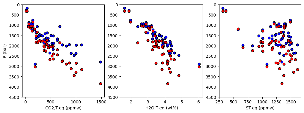
And we can plot the comparison below: default options in red, our options in blue.
[21]:
fig, (ax1, ax2, ax3) = plt.subplots(1, 3, figsize=(12,4))

# Plotting data

data1 = results1

ax1.plot(data1['CO2T-eq_ppmw'],
         data1['P_bar'], 'ok', mfc='blue')
ax2.plot(data1['H2OT-eq_wtpc'],
         data1['P_bar'], 'ok', mfc='blue')
ax3.plot(data1['ST_ppmw'],
         data1['P_bar'], 'ok', mfc='blue')

data1 = results2

ax1.plot(data1['CO2T-eq_ppmw'],
         data1['P_bar'], 'ok', mfc='red')
ax2.plot(data1['H2OT-eq_wtpc'],
         data1['P_bar'], 'ok', mfc='red')
ax3.plot(data1['ST_ppmw'],
         data1['P_bar'], 'ok', mfc='red')

ax1.set_xlabel('CO2,T-eq (ppmw)')
ax2.set_xlabel('H2O,T-eq (wt%)')
ax3.set_xlabel('ST-eq (ppmw)')
ax1.set_ylabel('P (bar)')
ax1.set_ylim([4500, 0])
ax2.set_ylim([4500, 0])
ax3.set_ylim([4500, 0])
[21]:
(4500.0, 0.0)