This page was generated from
docs/Examples/5a marianas.ipynb.
Interactive online version:
![]() .
.
5a. Full workflow: Marianas arc data
Here’s an example of a full workflow to explore melt inclusion and matrix glass data using VolFe. We’ll calculate saturation pressures, degassing paths, isobars, and fO2 from sulfur content from a single csv file in one notebook. We also compare to some of the other degassing tools available. This example is used in Hughes et al. (pre-print).
Python set-up
First we need to import a few Python packages (including VolFe). You need to install VolFe (and the other packages such as ThermoBar) once on your machine. If you haven’t yet, uncomment the line below (remove the # for the lines beginning !pip).
[1]:
# Install VolFe and Thermobar on your machine if you have not done so already. Remove the # from lines below to do this (don't remove the # from this line!).
# !pip install VolFe
# !pip install Thermobar
# !pip install VESIcal
[2]:
# import python packages
import pandas as pd
import numpy as np
import VolFe as vf
import Thermobar as tb
import VESIcal as vc
import matplotlib.pyplot as plt
c:\Users\ehughes\AppData\Local\miniforge3\envs\volfe-dev\Lib\site-packages\VESIcal\calculate_classes.py:7: UserWarning:

 WARNING: Thermoengine is not installed. MagmaSat model will not function. A model name must be given when performing any calculation as model='some-model-name'.
  from VESIcal.models import magmasat
Check version numbers
[3]:
# VolFe
vf.__version__
[3]:
'0.4.1'
[4]:
# Thermobar
tb.__version__
[4]:
'1.0.53'
[5]:
# VESIcal
vc.__version__
[5]:
'1.2.10'
Import data
First we will load our data from a csv file. We’ll use the examples_marianas csv in files again from Brounce et al. (2014, 2016) and Kelley & Cottrell (2012).
[6]:
my_analyses = pd.read_csv("../files/example_marianas.csv") # load data
Calculate temperature using Thermobar
All VolFe calculations require a temperature. We calculate temperature for each glass analysis using eq. (14) from Putirka (2008), which depends on melt composition including water but not pressure, using ThermoBar (Wieser et al. 2022). This is then added to the dataframe of compositions.
[7]:
# renames melt composition headers to be comparible with Thermobar
my_analyses_tb = my_analyses.rename(columns = {"SiO2":"SiO2_Liq","TiO2":"TiO2_Liq","Al2O3":"Al2O3_Liq","FeOT":"FeOt_Liq","MnO":"MnO_Liq","MgO":"MgO_Liq","CaO":"CaO_Liq",
                                               "Na2O":"Na2O_Liq","K2O":"K2O_Liq","P2O5":"P2O5_Liq","H2O":"H2O_Liq"})
# calculates T using Thermobar based on eq. (14) from Putirka (2008) and converts to 'C
T_C_all = tb.calculate_liq_only_temp(liq_comps=my_analyses_tb, equationT="T_Put2008_eq14")-273.15
# adds temperatures to original dataframe
my_analyses.insert(1,"T_C",T_C_all)
Later on, we also require the error associated with the temperature - the reported SEE for this thermometer is 51 ‘C, which we add to the dataframe as well as a column stating the error is absolute rather than than relative.
[8]:
my_analyses['T_C_sd'] = 51.
my_analyses['T_C_sd_type'] = 'A'
Calculate the pressure of vapor-saturation
Now we can calculate the pressure of vapor saturation for all the analyses in the file using the default models in VolFe.
[9]:
# run calculation
pvsat = vf.calc_Pvsat(my_analyses)
# save results
pvsat.to_csv('../files/marianas_pvsat.csv', index=False, header=True)
# load result
pvsat = pd.read_csv("../files/marianas_pvsat.csv")
Calculate the fO2 from the sulfur content
Instead of using the Fe3+/FeT measured in the glass to calculate fO2, we can instead use the measured S content and compare it too the S2-CSS.
[10]:
# run calculation
fO2fromS = vf.calc_melt_S_oxybarometer(my_analyses)
# save results
fO2fromS.to_csv('../files/marianas_fO2fromS.csv', index=False, header=True)
# load result
fO2fromS = pd.read_csv("../files/marianas_fO2fromS.csv")
Influence of melt composition errors
Next we look at how errors in the melt composition might influence the calculations we have done: pvsat and fO2 from measured S. We use a Monte Carlo approach to calculate 100 potential compositions of each MI/SPG to see how that effects our calculations.
[11]:
# run calculation
pvsat_all_errors = vf.calc_comp_error_function(my_analyses,iterations=100,function='calc_Pvsat')
# save results
pvsat_all_errors.to_csv('../files/marianas_pvsat_all_errors.csv', index=False, header=True)
# load result
pvsat_all_errors = pd.read_csv("../files/marianas_pvsat_all_errors.csv")
100%|██████████| 51/51 [40:38<00:00, 47.81s/it]
[12]:
# run calculation
S2fO2_all_errors = vf.calc_comp_error_function(my_analyses,iterations=100,function='calc_melt_S_oxybarometer')
# save results
S2fO2_all_errors.to_csv('../files/marianas_S2fO2_all_errors.csv', index=False, header=True)
# load result
S2fO2_all_errors = pd.read_csv("../files/marianas_S2fO2_all_errors.csv")
100%|██████████| 51/51 [1:27:30<00:00, 102.96s/it]
Calculate isobars
We can also calculate isobars for Ala02-16A but we need to change the “insolubles” option to “H2O-CO2 only” to do this.
[13]:
# change just the "COH_species" option to "H2O-CO2 only"
my_models = [['COH_species','H2O-CO2 only']]
# turn "my_models" to dataframe with correct column headers and indexes
my_models = vf.make_df_and_add_model_defaults(my_models)
# calculate isobars for Ala01-16A which is run 29 in the csv starting at 1000 bars, ending at 4000 bars at 1000 bar intervals
isobars = vf.calc_isobar(my_analyses,run=29,models=my_models,initial_P=1000.,final_P=5000.,step_P=1000.)
# save results
isobars.to_csv('../files/marianas_isobars.csv', index=False, header=True)
# load result
isobars = pd.read_csv("../files/marianas_isobars.csv")
# split into each pressure for plotting
isobar1000 = isobars[isobars["P_bar"]==1000.]
isobar2000 = isobars[isobars["P_bar"]==2000.]
isobar3000 = isobars[isobars["P_bar"]==3000.]
isobar4000 = isobars[isobars["P_bar"]==4000.]
isobar5000 = isobars[isobars["P_bar"]==5000.]
Calculate de/regassing paths
Closed-system, melt-only, degassing
Next we can run a closed-system degassing calculation starting from Ala02-16A, using the default options.
[14]:
# run calculation
degassing_closed_1 = vf.calc_gassing(my_analyses,run=29)
# save result
degassing_closed_1.to_csv('../files/marianas_degas_closed_1.csv', index=False, header=True)
# load result
degassing_closed_1 = pd.read_csv("../files/marianas_degas_closed_1.csv")
100%|█████████▉| 3199.0/3200 [00:29<00:00, 107.38it/s]
Closed-system, melt+vapor, degassing
But it probably had more CO2 to start with… so we can run a closed-system degassing calculation assuming the initial melt contained 2 wt% CO2.
[15]:
# 'bulk composition' to 'melt+vapor_initialCO2'
my_models = [['bulk_composition',"melt+vapor_initialCO2"]]

# turn to dataframe with correct column headers and indexes
my_models = vf.make_df_and_add_model_defaults(my_models)

# run calculation
degassing_closed_2 = vf.calc_gassing(my_analyses,run=29,models=my_models)
# save result
degassing_closed_2.to_csv('../files/marianas_degas_closed_2.csv', index=False, header=True)
# load result
degassing_closed_2 = pd.read_csv("../files/marianas_degas_closed_2.csv")
100%|█████████▉| 3199.0/3200 [00:21<00:00, 147.70it/s]
Closed-system, melt+gas, regassing
… and regas along the same path to see how it would have evolved at higher pressures before the melt inclusion was formed.
[16]:
# change to regas and melt+vapor_initialCO2
my_models = [['gassing_direction','regas'],['bulk_composition',"melt+vapor_initialCO2"]]

# turn to dataframe with correct column headers and indexes
my_models = vf.make_df_and_add_model_defaults(my_models)

# run calculation
regassing_closed_2 = vf.calc_gassing(my_analyses,run=29,models=my_models)
# save result
regassing_closed_2.to_csv('../files/marianas_regas_closed_2.csv', index=False, header=True)
# load result
regassing_closed_2 = pd.read_csv("../files/marianas_regas_closed_2.csv")
1800.0it [00:05, 325.56it/s]
Open-system degassing
And we can compare it to open-system degassing…
[17]:
# change just the "COH_species" option to "H2O-CO2 only"
my_models = [['gassing_style','open']]

# turn to dataframe with correct column headers and indexes
my_models = vf.make_df_and_add_model_defaults(my_models)

# run calculation
degassing_open = vf.calc_gassing(my_analyses,run=29,models=my_models)
# save result
degassing_open.to_csv('../files/marianas_degas_open.csv', index=False, header=True)
# load result
degassing_open = pd.read_csv("../files/marianas_degas_open.csv")
52%|█████▏ | 1673.0/3241 [16:08<15:07, 1.73it/s]
Open-system regassing
… and open-system regassing …
[18]:
# change just the "COH_species" option to "H2O-CO2 only"
my_models = [['gassing_style','open'],['gassing_direction','regas']]

# turn to dataframe with correct column headers and indexes
my_models = vf.make_df_and_add_model_defaults(my_models)

# run calculation
regassing_open = vf.calc_gassing(my_analyses,run=29,models=my_models)
# save result
regassing_open.to_csv('../files/marianas_regas_open.csv', index=False, header=True)
# load result
regassing_open = pd.read_csv("../files/marianas_regas_open.csv")
1759.0it [20:11, 1.45it/s]
Comparison to other tools
We can compare the results of the closed-system, melt-only, degassing calculation to the results from other tools that are available.
VESIcal (Iacovino et al., 2021)
Using the VolatileCalc model (Newman & Lowerstern, 2022), which is closest to the model dependent variable options used in the VolFe calculation.
[19]:
my_sample = vc.Sample({'SiO2':  43.97,
 'TiO2':   0.7,
 'Al2O3': 19.09,
 'Fe2O3':  0.,
 'Cr2O3':  0.0,
 'FeO':    9.36,
 'MnO':    0.22,
 'MgO':    6.76,
 'NiO':    0.0,
 'CoO':    0.0,
 'CaO':    13.28,
 'Na2O':   1.46,
 'K2O':    0.37,
 'P2O5':   0.11,
 'H2O':    4.32,
 'CO2':    0.0999})

# run degassing calculation
vesical_volatilecalc = vc.calculate_degassing_path(sample=my_sample,temperature=1111.,model='Dixon').result
# save result
vesical_volatilecalc.to_csv('../files/comparison/vesical_volatilecalc.csv', index=False, header=True)
# load result
vesical_volatilecalc = pd.read_csv("../files/comparison/vesical_volatilecalc.csv")
Sulfur_X (Ding et al., 2023)
Initial conditions and model options can be found in ‘main_Fuego.py’ and ‘melt_composition.py’.
[20]:
sulfur_X = pd.read_csv("../files/comparison/sulfur_X.csv") # load data
CHOSETTO (Moretti et al., 2003; Moretti & Papale, 2004)
Initial conditions and model options can be found in “chosetto.ctr” and “chosetto.dat”. The original output (chosetto.out) was converted to csv, D was replaced with E throughout, and column headers were added.
[21]:
chosetto = pd.read_csv("../files/comparison/chosetto.csv") # load data
[22]:
x = (chosetto['FeO_Fe2O3']*2.*159.69)/71.844
chosetto_Fe3_FeT = 1.-(x/(x+1.))
EVo (Liggins et al., 2022, 2020)
Initial conditions can be found in ‘env_ery.yaml’ and ‘chem_ery.yaml’.
[23]:
evo = pd.read_csv("../files/comparison/dgs_output_basalt_COHS_closed_1384K.csv") # load data
Plotting
Finally, we can plot all everything!
[24]:
fig, (ax1,ax2,ax3,ax4) = plt.subplots(1, 4, figsize=(16,4))

# TAS
ax1.errorbar(my_analyses['SiO2'], y=(my_analyses['K2O']+my_analyses['Na2O']),
             xerr=((2.*my_analyses["SiO2_sd"])*my_analyses["SiO2"]), yerr=(2*(my_analyses["Na2O_sd"]**2+my_analyses["K2O_sd"]**2.)**0.5)*(my_analyses["K2O"]+my_analyses["Na2O"]),
             fmt='o')
ax1.set_ylabel('N2O+K2O (wt%)')
ax1.set_xlabel('SiO2 (wt%)')

# H2O-CO2
for x in [isobar1000,isobar2000,isobar3000,isobar4000,isobar5000]:
    ax2.plot(x["H2O_wtpc"], x["CO2_ppm"], '-k')
ax2.errorbar(my_analyses['H2O'], y=my_analyses['CO2ppm'], xerr=(2.*my_analyses['H2O_sd']), yerr=(2*my_analyses["CO2ppm_sd"]), fmt='o', zorder=0)
ax2.plot(degassing_closed_1['H2OT-eq_wtpc'], degassing_closed_1['CO2T-eq_ppmw'], '-b', linewidth=3.)
ax2.plot(degassing_closed_2['H2OT-eq_wtpc'], degassing_closed_2['CO2T-eq_ppmw'], '-r', linewidth=3.)
ax2.plot(regassing_closed_2['H2OT-eq_wtpc'], regassing_closed_2['CO2T-eq_ppmw'], ':r', linewidth=3.)
ax2.plot(regassing_open['H2OT-eq_wtpc'], regassing_open['CO2T-eq_ppmw'], ':b', linewidth=3.)
ax2.plot(degassing_open['H2OT-eq_wtpc'], degassing_open['CO2T-eq_ppmw'], '--b', linewidth=3.)
ax2.set_xlabel('H2OT-eq (wt%)')
ax2.set_ylabel('CO2-eq (ppmw)')
ax2.set_ylim([0,2500])
ax2.set_xlim([0,6.1])

# Fe3+/FeT-ST
ax3.errorbar(my_analyses['Fe3FeT'], y=my_analyses['STppm'], xerr=(2.*my_analyses['Fe3FeT_sd']), yerr=(2*my_analyses["STppm_sd"]), fmt='o', zorder=0)
ax3.plot(degassing_closed_1['Fe3+/FeT'], degassing_closed_1['ST_ppmw'], '-b', linewidth=3.)
ax3.plot(degassing_closed_2['Fe3+/FeT'], degassing_closed_2['ST_ppmw'], '-r', linewidth=3.)
ax3.plot(regassing_closed_2['Fe3+/FeT'], regassing_closed_2['ST_ppmw'], ':r', linewidth=3.)
ax3.plot(regassing_open['Fe3+/FeT'], regassing_open['ST_ppmw'], ':b', linewidth=3.)
ax3.plot(degassing_open['Fe3+/FeT'], degassing_open['ST_ppmw'], '--b', linewidth=3.)
ax3.set_xlabel('Fe3+/FeT')
ax3.set_ylabel('ST (ppmw)')


# H2O-ST
ax4.errorbar(my_analyses['H2O'], y=my_analyses['STppm'], xerr=(2.*my_analyses['H2O_sd']), yerr=(2*my_analyses["STppm_sd"]), fmt='o', zorder=0)
ax4.plot(degassing_closed_1['H2OT-eq_wtpc'], degassing_closed_1['ST_ppmw'], '-b', linewidth=3.)
ax4.plot(degassing_closed_2['H2OT-eq_wtpc'], degassing_closed_2['ST_ppmw'], '-r', linewidth=3.)
ax4.plot(regassing_closed_2['H2OT-eq_wtpc'], regassing_closed_2['ST_ppmw'], ':r', linewidth=3.)
ax4.plot(regassing_open['H2OT-eq_wtpc'], regassing_open['ST_ppmw'], ':b', linewidth=3.)
ax4.plot(degassing_open['H2OT-eq_wtpc'], degassing_open['ST_ppmw'], '--b', linewidth=3.)
ax4.set_xlabel('H2O-eq (wt%)')
ax4.set_ylabel('ST (ppm)')
fig.tight_layout(pad=1.0)

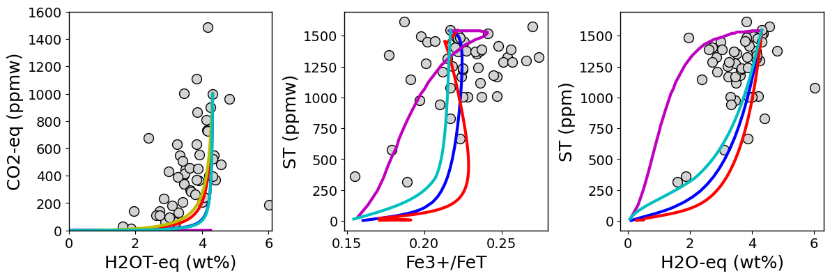
[25]:
fig, (ax1,ax2,ax3) = plt.subplots(1, 3, figsize=(12,4))

# H2O-CO2
ax1.plot(my_analyses['H2O'], my_analyses['CO2ppm'], 'ok', mfc='lightgrey')
ax1.plot(degassing_closed_1['H2OT-eq_wtpc'], degassing_closed_1['CO2T-eq_ppmw'], '-b', linewidth=3.)
ax1.plot(sulfur_X['wH2O_melt'], sulfur_X['wCO2_melt'], '-r', linewidth=3.)
ax1.plot(chosetto['wm_H2O']*100., chosetto['wm_CO2']*100000., '-m', linewidth=3.)
ax1.plot(vesical_volatilecalc['H2O_liq'], vesical_volatilecalc['CO2_liq']*10000., '-y', linewidth=3.)
ax1.plot(evo['H2O_melt'], evo['CO2_melt']*10000., '-c', linewidth=3.)
ax1.set_xlabel('H2OT-eq (wt%)')
ax1.set_ylabel('CO2-eq (ppmw)')
ax1.set_ylim([0,1600])
ax1.set_xlim([0,6.1])

# Fe3+/FeT-ST
ax2.plot(my_analyses['Fe3FeT'], my_analyses['STppm'], 'ok', mfc='lightgrey')
ax2.plot(degassing_closed_1['Fe3+/FeT'], degassing_closed_1['ST_ppmw'], '-b', linewidth=3.)
ax2.plot(sulfur_X['ferric_ratio'], sulfur_X['wS_melt'], '-r', linewidth=3.)
ax2.plot(chosetto_Fe3_FeT, chosetto['wm_S']*1000000., '-m', linewidth=3.)
ax2.plot(evo['Fe3FeT'], evo['Stot_melt']*10000., '-c', linewidth=3.)
ax2.set_xlabel('Fe3+/FeT')
ax2.set_ylabel('ST (ppmw)')


# H2O-ST
ax3.plot(my_analyses['H2O'], my_analyses['STppm'], 'ok', mfc='lightgrey')
ax3.plot(degassing_closed_1['H2OT-eq_wtpc'], degassing_closed_1['ST_ppmw'], '-b', linewidth=3.)
ax3.plot(sulfur_X['wH2O_melt'], sulfur_X['wS_melt'], '-r', linewidth=3.)
ax3.plot(chosetto['wm_H2O']*100., chosetto['wm_S']*1000000., '-m', linewidth=3.)
ax3.plot(evo['H2O_melt'], evo['Stot_melt']*10000., '-c', linewidth=3.)
ax3.set_xlabel('H2O-eq (wt%)')
ax3.set_ylabel('ST (ppm)')
fig.tight_layout(pad=1.0)
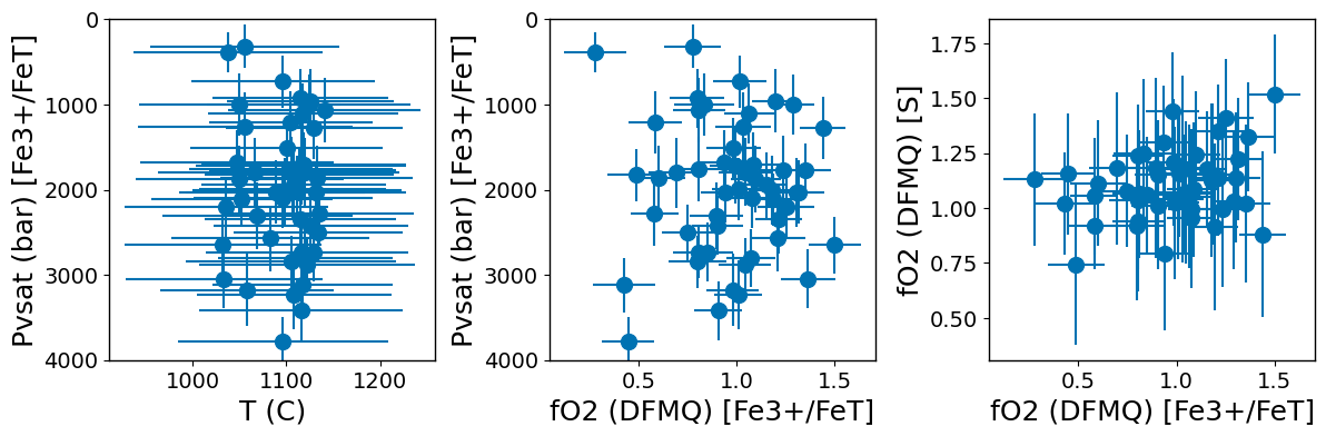
[26]:
fig, (ax1,ax2,ax3) = plt.subplots(1, 3, figsize=(12,4))

# P-T
ax1.errorbar(pvsat_all_errors['T_C'], y=pvsat_all_errors['P_bar'],
             xerr=(2.*pvsat_all_errors['T_C_sd']), yerr=(2*pvsat_all_errors["P_bar_sd"]), fmt='o', zorder=0)
ax1.set_ylabel('Pvsat (bar) [Fe3+/FeT]')
ax1.set_xlabel('T (C)')
ax1.set_ylim([4000,0])

# P-fO2[Fe3+/FeT]
ax2.errorbar(pvsat_all_errors['fO2_DFMQ'], y=pvsat_all_errors['P_bar'],
             xerr=(2.*pvsat_all_errors['fO2_DFMQ_sd']), yerr=(2*pvsat_all_errors["P_bar_sd"]), fmt='o', zorder=0)
ax2.set_ylabel('Pvsat (bar) [Fe3+/FeT]')
ax2.set_xlabel('fO2 (DFMQ) [Fe3+/FeT]')
ax2.set_ylim([4000,0])

# fO2[S]-fO2[Fe3+/FeT]
ax3.errorbar(pvsat_all_errors['fO2_DFMQ'], y=S2fO2_all_errors['fO2_DFMQ_sulf'],
             xerr=(2.*pvsat_all_errors['fO2_DFMQ_sd']), yerr=(2*S2fO2_all_errors['fO2_DFMQ_sulf_sd']), fmt='o', zorder=0)
ax3.set_ylabel('fO2 (DFMQ) [S]')
ax3.set_xlabel('fO2 (DFMQ) [Fe3+/FeT]')

fig.tight_layout(pad=1.0)
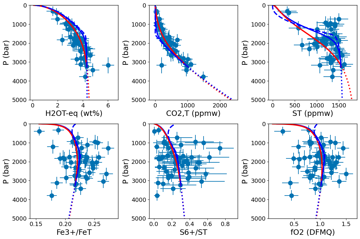
[27]:
fig, ((ax1,ax2,ax3),(ax4,ax5,ax6)) = plt.subplots(2, 3, figsize=(12,8))

for x in [ax1,ax2,ax3,ax4,ax5,ax6]:
    if x == ax1:
        value = 'H2OT-eq_wtpc'
        x.set_xlabel('H2OT-eq (wt%)')
    elif x == ax2:
        value = 'CO2T-eq_ppmw'
        x.set_xlabel('CO2,T (ppmw)')
    elif x == ax3:
        value = 'ST_ppmw'
        x.set_xlabel('ST (ppmw)')
    elif x == ax4:
        value = 'Fe3+/FeT'
        x.set_xlabel('Fe3+/FeT')
    elif x == ax5:
        value = 'S6+/ST'
        x.set_xlabel('S6+/ST')
    elif x == ax6:
        value = 'fO2_DFMQ'
        x.set_xlabel('fO2 (DFMQ)')
    x.errorbar(pvsat_all_errors[value], y=pvsat_all_errors['P_bar'], xerr=(2.*pvsat_all_errors[value+'_sd']), yerr=(2*pvsat_all_errors["P_bar_sd"]), fmt='o', zorder=0)
    x.plot(degassing_closed_1[value], degassing_closed_1['P_bar'], '-b', linewidth=3.)
    x.plot(degassing_closed_2[value], degassing_closed_2['P_bar'], '-r', linewidth=3.)
    x.plot(regassing_closed_2[value], regassing_closed_2['P_bar'], ':r', linewidth=3.)
    x.plot(regassing_open[value], regassing_open['P_bar'], ':b', linewidth=3.)
    x.plot(degassing_open[value], degassing_open['P_bar'], '--b', linewidth=3.)
    x.set_ylabel('P (bar)')
    x.set_ylim([5000,0])

fig.tight_layout(pad=1.0)
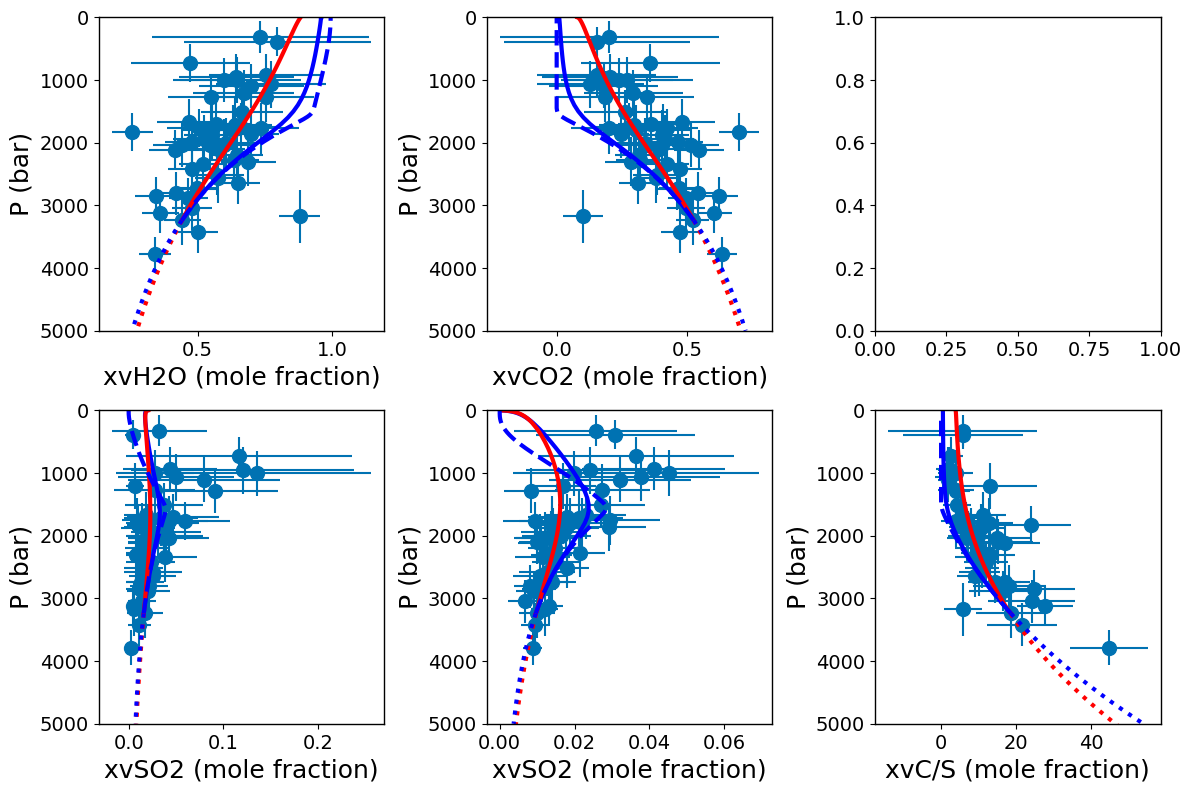
[28]:
fig, ((ax1,ax2,ax3),(ax4,ax5,ax6)) = plt.subplots(2, 3, figsize=(12,8))

for x in [ax1,ax2,ax4,ax5,ax6]:
    if x == ax1:
        value = 'xgH2O_mf'
        x.set_xlabel('xvH2O (mole fraction)')
    elif x == ax2:
        value = 'xgCO2_mf'
        x.set_xlabel('xvCO2 (mole fraction)')
    elif x == ax4:
        value = 'xgSO2_mf'
        x.set_xlabel('xvSO2 (mole fraction)')
    elif x == ax5:
        value = 'xgH2S_mf'
        x.set_xlabel('xvSO2 (mole fraction)')
    elif x == ax6:
        value = 'xgC_S_mf'
        x.set_xlabel('xvC/S (mole fraction)')
    x.errorbar(pvsat_all_errors[value], y=pvsat_all_errors['P_bar'], xerr=(2.*pvsat_all_errors[value+'_sd']), yerr=(2*pvsat_all_errors["P_bar_sd"]), fmt='o', zorder=0)
    x.plot(degassing_closed_1[value], degassing_closed_1['P_bar'], '-b', linewidth=3.)
    x.plot(degassing_closed_2[value], degassing_closed_2['P_bar'], '-r', linewidth=3.)
    x.plot(regassing_closed_2[value], regassing_closed_2['P_bar'], ':r', linewidth=3.)
    x.plot(regassing_open[value], regassing_open['P_bar'], ':b', linewidth=3.)
    x.plot(degassing_open[value], degassing_open['P_bar'], '--b', linewidth=3.)
    x.set_ylabel('P (bar)')
    x.set_ylim([5000,0])

fig.tight_layout(pad=1.0)