This page was generated from docs/Examples/4a. other_fug_coeff.ipynb. Interactive online version: .

Python Notebook Download

4a. Calculate fugacity coefficients

This allows you to calculate the fugacity coefficient for all vapor species in the CHOSX system at a given P and T.

It can be run for multiple sets of conditions defined in the input data frame or loaded from a csv file.

Python set-up

You need to install VolFe once on your machine, if you haven’t yet. Then we need to import a few Python packages (including VolFe).

# Install VolFe on your machine. Don't remove the # from this line!
# pip install VolFe # Remove the first # in this line if you have not installed VolFe on your machine before.

# import python packages
import pandas as pd
import matplotlib.pyplot as plt
import VolFe as vf

Conditions from dataframe

Define the inputs

This first example is for a single set of conditions defined in a dataframe.

# Define conditions T as a dictionary.
my_analysis = {'Sample':'test',
           'T_C': 1200., # Temperature in 'C
           'P_bar':1000.} # Pressure in bar

# Turn the dictionary into a pandas dataframe, setting the index to 0.
my_analysis = pd.DataFrame(my_analysis, index=[0])

We’ll use the default options

# print default options in VolFe
print(vf.default_models)

                            option
type
COH_species     yes_H2_CO_CH4_melt
H2S_m                         True
species X                       Ar
Hspeciation                   none
fO2                       Kress91A
...                            ...
error                          0.1
print status                 False
output csv                    True
setup                        False
high precision               False

[78 rows x 1 columns]

Run the calculation

And this runs the calculation

vf.calc_fugacity_coefficients(my_analysis)

	Sample	P_bar	T_C	yO2	yH2	yH2O	yS2	ySO2	yH2S	yCO2	...	y_H2S opt	y_H2 opt	y_O2 opt	y_S2 opt	y_CO opt	y_CH4 opt	y_H2O opt	y_OCS opt	y_X opt	Date
0	test	1000.0	1200.0	1.209858	1.126166	1.004254	1.191327	1.206456	1.489942	1.265765	...	Shi92_Hughes24	Shaw64	Shi92	Shi92	Shi92	Shi92	Holland91	Shi92	ideal	2025-02-02 10:12:53.052359

1 rows × 26 columns

Conditions from file

Import data

We’ll show an example by loading from the csv file found in files.

# Read csv to define melt composition
my_analyses = pd.read_csv("../files/inputs_y.csv")

Run the calculation

And below runs the calculation

results = vf.calc_fugacity_coefficients(my_analyses)

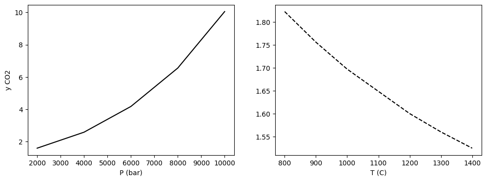
Plotting

And we can plot them - this is an example for CO2

fig, (ax1, ax2) = plt.subplots(1, 2, figsize=(12,4))

data1 = results[results['P_bar'] == 2000.] # 2000 bar
data2 = results[results['T_C'] == 1200.] # 1200 'C

# Plotting results
ax1.plot(data2['P_bar'], data2['yCO2'], '-k')
ax2.plot(data1['T_C'], data1['yCO2'], '--k')

ax1.set_xlabel('P (bar)')
ax2.set_xlabel('T (C)')
ax1.set_ylabel('y CO2')

Text(0, 0.5, 'y CO2')